Authors: Wanxiong Cai (RUB)

The following REPAIRS toolbox is available under the CC-BY licence (Creative- Commons:  https://creativecommons.org/). This implies that others are free to share and adapt our works under the condition that appropriate credit to the original contribution (provide the name of the REPAIRS consortium and the name the authors of the toolbox when available, and a link to the original material) is given and indicate if changes were made to the original work. 

Linear regression for determining the Jacobian matrix in UCM analysis 

Overview 
This is a part of the UCM toolbox that introduces the method of utilizing linear regression to determine the Jacobian matrix in UCM analysis. The general procedure of UCM analysis will not be covered here. 

Motivation 
The typical UCM analysis involves calculating the Jacobian from a geometric model that connects joint positions and segment lengths to the end-effector position. Even though there’s usually a formal geometric model, it can be too complicated to solve analytically in some cases, like when the hand is fixed on an external object that restricts movement (de Freitas, S.M.S.F. and Scholz, J.P., 2010.).  
In other cases, some physiological variables other than joint angles make the estimation of Jacobian even more difficult. For instance, joint torque is driven by multiple muscles on the corresponding joint, and if we want to conduct UCM analysis on this scenario where joint torque is the task variable and muscle activity is the elemental variable, we need to derive a very complex model. This model involves a series of non-linear equations describing several biomechanical processes where the output of the previous one is the input of the next one, which includes dynamics of muscle activation, muscle force generation, muscle-tendon dynamics, and finally, the joint torque generation module. If we nest these modules together, we will obtain a complicated system of equations, making it impossible to write a single clean Jacobian matrix.  
To address similar problems, researchers have estimated the Jacobian using linear regression between EMG patterns and a task-level variable, such as the center of foot pressure (Krishnamoorthy et al., 2003).
Besides the simplicity of linear regression for Jacobian matrix deriving, researchers have also argued that linear regression can be a more preferred analytical method in the data of goal-directed reaching tasks (Tuitert. et al., 2019). This study demonstrates that the linear model created with the regression method provided a more accurate description of the data, because linear regression incorporates the distribution of the data across repetitions into the linear model, whereas the analytical method considers only the averages. 

General procedure  

1. Determine elemental variables and task variables. 

2. Collect data and conduct linear regression. 

3. Evaluate the performance of the linear model. 

4. Construct the Jacobian matrix with coefficients given by regression.  

5. Solve the null space. 

6. Follow the common procedure of variance computation in UCM analysis. 

    Example 
We use a classical planar arm model to illustrate the usage of linear regression, which can be used in experiments like goal-directed arm-reaching tasks.  

As shown in the figure above, l₁, l₂ , l₃ are the link lengths, θ₁ , θ ₂ , θ ₃ are the local joint angles. In a typical UCM analysis, we write down the geometric model relating the position (x,y) of the end effector to the joint angles: 

The Jacobian matrix is given by 

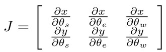
where each entry is a partial derivate of the geometric equation in an analytic method, for instance: 

This process can be even more straightforward with the linear regression method. First, we write down a linear model:

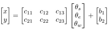
After we regress the model with data from experiments, the Jacobian matrix is simply the coefficient matrix obtained. However, the performance of the linear model should always be evaluated before null space computation to ensure the approximation is good enough for UCM analysis. This can be done by calculating the amount of residual error of the prediction using the linear model compared with the measured positions of the end effector. Moreover, it is advised to always check properties of the residuals to get an idea of the quality of the fit.
We implement the example with surrogate data in MATLAB.   
First, we generate some joint angles:

theta_s = linspace(pi/6, pi/2-pi/12, 20);
theta_e = linspace(pi-pi/3, pi/6, 20);
theta_w = linspace(0, pi/12, 20);

Then, we compute the position of the end effector using the geometrical model:

l_1 = 0.33;
l_2 = 0.26;
l_3 = 0.12;
position_x = l_1*cos(theta_s) + l_2*cos(theta_s + theta_e) + l_3 * cos(theta_s + theta_e + theta_w);
position_y = l_1*sin(theta_s) + l_2*sin(theta_s + theta_e) + l_3 * sin(theta_s + theta_e + theta_w);

Finally, we regress the positions (x, y) on joint angles:

mat_theta = [theta_s; theta_e; theta_w]’;
X = [ones(size(mat_theta, 1), 1) mat_theta];
b1 = regress(position_x’, X);
b2 = regress(position_y’, X);

Now, we can check the performance of the linear model by calculating the R²:

fitX = X * b1;
fitY = X * b2;
SS_res = sum(([position_x’ position_y’] – [fitX fitY]).^2);  % Residual sum of squares
SS_tot = sum(([position_x’ position_y’] – mean([position_x’ position_y’])).^2);  % Total sum of squares
R_squared = 1 – SS_res / SS_tot;

References
Krishnamoorthy, V., Latash, M. L., Scholz, J. P., & Zatsiorsky, V. M. (2003). Muscle synergies during shifts of the center of pressure by standing persons. Experimental brain research, 152, 281-292.
de Freitas, S. M. S. F., & Scholz, J. P. (2010). A comparison of methods for identifying the Jacobian for uncontrolled manifold variance analysis. Journal of biomechanics, 43(4), 775-777.
Tuitert, I., Valk, T. A., Otten, E., Golenia, L., & Bongers, R. M. (2019). Comparing different methods to create a linear model for Uncontrolled Manifold Analysis. Motor Control, 23(2), 189-204.