Authors: Jan Thomas (UMCG), Wanxiong Cai (RUB)

The following REPAIRS toolbox is available under the CC-BY licence (Creative- Commons:  https://creativecommons.org/). This implies that others are free to share and adapt our works under the condition that appropriate credit to the original contribution (provide the name of the REPAIRS consortium and the name the authors of the toolbox when available, and a link to the original material) is given and indicate if changes were made to the original work. 

Human movements, from grasping a cup to juggling, require numerous muscles working together to achieve smooth and precise movements. A fundamental question in motor control is how the nervous system takes full advantage of so many muscles to perform stable and flexible movements.
Muscle synergies offer a potential solution: muscles are activated together as groups called synergies. In the muscle synergy approach to motor control, these synergies follow from the modular organization of the spinal cord. A module in the spinal cord generates a specific, functional movement pattern by imposing a specific pattern of muscle activation, called muscle synergies. These synergies reduce the complexity of controlling each muscle individually, providing a more efficient way of motor control. This principle motivated researchers to develop methods to analyze muscle synergies effectively.
Muscles receive “commands” encoded by electrical signals sent by neurons and contract, which also rely on electrical activity in muscle fibers. Electromyography (EMG) is a technique for measuring muscle electrical activity, and it is the most used method for quantifying muscle contractions. Researchers can decompose these signals into muscle synergies using methods like Non-Negative Matrix Factorization (NNMF) after EMG signal processing.
The EMG data, which captures the electrical activity of muscles, is organized into a matrix. NNMF decomposes this matrix into two smaller matrices: one representing muscle synergies (or modes), which are groups of muscles that work together, and the other representing the activation patterns (temporal activations) of these synergies over time. This decomposition allows us to identify and analyze the underlying muscle coordination patterns. In an example shown below, there are two synergies where each muscle contributes differently in the blue synergy and the red synergy. The nervous system gives corresponding time courses of activation for each synergy, producing the final muscle activation patterns. The codes for this example have been attached later in this document.

This document introduces the general pipeline of EMG signal processing for/and NNMF analysis, highlighting their applications in two classical motor control tasks: isometric force production and planar reaching.

1. Virtual Isometric Task

Isometric force production in goal-directed tasks involves generating muscle force without any actual movement of the joints. This type of task is designed to assess and train the ability to control muscle force precisely and maintain a specific level of contraction. The task is oriented towards achieving a specific objective. This could involve maintaining a constant force level, matching a target force, or varying force output according to a predefined pattern. The continuous virtual task involves mapping the muscle activities onto a virtual object. NNMF breaks down EMG data collected from muscles during isometric tasks into simpler components. This decomposition allows us to observe how these patterns change as a participant learns or improves in performing the isometric task. By comparing these patterns across different sessions, NNMF helps track the stability and adaptation of muscle coordination.

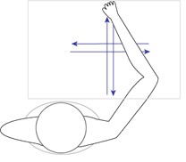
2. Planar Reaching Task

The planar reaching task involves moving the arm to shift the hand from one location to another. The degrees of freedom of the wrist and fingers are often frozen, so there are only movements of the elbow and shoulder joint. The muscles on each joint can play different roles, which activate at different times during the movement. For example, in a fast arm movement, there is a propulsion phase and a braking phase, where different groups of muscles activate. Moreover, some bi-articular muscles also perform differently than their mono-articular synergists due to the interaction between joints. If we want to understand the specific functions of these muscles and their coordination, only plotting out their average waveform is intuitive but not very insightful. NNMF allows us to extract these synergies and display the contribution of each muscle quantitatively.

Pre-Processing:
The website by Roberto Merletti provides a good background on EMG. We need a suitable EMG system to record the raw EMG signals. To capture the muscle activity accurately, ensure a sampling rate of at least 1000 Hz.

Artifact Removal:
A median filter can be used to remove transient noise and motion artifacts. An appropriate window size is chosen depending on whether the filter is used for high-frequency noise removal or motion artifact removal. Then, the median and median absolute deviation are calculated for the window size. Then, outliers are identified as values whose deviations exceed a certain threshold.

Filtering:
The resulting EMG data can be band-pass filtered using a 4th-order Butterworth filter with a frequency range (e.g., 20-500 Hz) to remove noise and retain relevant signal components.

 Rectification and Smoothening:
A 4th-order Butterworth low-pass filter with a cut-off frequency (e.g., 10 Hz) was applied to the rectified signals to determine the linear envelope, providing a smoothed version of the EMG signal.

Normalisation:
The amplitude of the EMG data for each muscle can then be normalized to the highest value across trials.

Time normalisation:
Data can be time-normalized to steps using cubic spline interpolation, ensuring uniformity in the time axis across different trials and sessions.

Part 1: MATLAB Codes with generated surrogate EMG:

fs = 1000; % Sampling rate in Hz

t = 0:1/fs:10; % Time vector (10 seconds of data)

emg_signal = 5.5 * sin(2 * pi * 50 * t) + 5.5 * sin(2 * pi * 120 * t);

% Add Gaussian noise

noise_gaussian = 0.5 * randn(size(t));

% Add motion artifacts (low frequency noise)

motion_artifact = 0.5 * sin(2 * pi * 1 * t);

% Combine EMG signal with noise artifacts

raw_emg = emg_signal + noise_gaussian + motion_artifact;

% Artifact Removal using Median Filter

window_size = 201; % Adjust as needed for high frequency noise or motion artifact

filtered_emg = medfilt1(raw_emg, window_size);

% Band-pass Filter (20-500 Hz) using 4th order Butterworth filter

lowcut = 20;

highcut = 499.99;

[b, a] = butter(4, [lowcut, highcut] / (fs / 2), ‘bandpass‘);

bandpassed_emg = filtfilt(b, a, filtered_emg);

rectified_emg = abs(bandpassed_emg);

% Low-pass Filter (10 Hz) using 4th order Butterworth filter for smoothing

cutoff = 10;

[d, c] = butter(4, cutoff / (fs / 2), ‘low‘);

smoothed_emg = filtfilt(d, c, rectified_emg);

% Normalization

max_value = max(smoothed_emg);

normalized_emg = smoothed_emg / max_value;

time_normalized_length = 1000; % Number of points in the time-normalized signal

original_time = t;

uniform_time=linspace(original_time(1),original_time(end),time_normalized_length);time_normalized_emg = spline (original_time, normalized_emg, uniform_time);

Part 2: MATLAB Codes for the example of muscle synergies

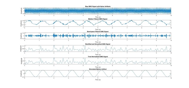
figure;

subplot(6, 1, 1);

plot(t, raw_emg);

title(‘Raw EMG Signal with Noise Artifacts’);

xlabel(‘Time (s)’);

ylabel(‘Amplitude’);

subplot(6, 1, 2);

plot(t, filtered_emg);

title(‘Median Filtered EMG Signal’);

xlabel(‘Time (s)’);

ylabel(‘Amplitude’);

subplot(6, 1, 3);

plot(t, bandpassed_emg);

title(‘Band-pass Filtered EMG Signal’);

xlabel(‘Time (s)’);

ylabel(‘Amplitude’);

subplot(6, 1, 4);

plot(t, smoothed_emg);

title(‘Rectified and Smoothed EMG Signal’);

xlabel(‘Time (s)’);

ylabel(‘Amplitude’);

subplot(6, 1, 5);

plot(uniform_time, time_normalized_emg);

title(‘Time Normalized EMG Signal’);

xlabel(‘Time (s)’);

ylabel(‘Amplitude’);

NNMF
The pre-processed EMG data (M_observed) can be decomposed using NNMF to identify muscle modes and their activation signals. NNMF decomposes the EMG data into two matrices: W (modes) and C (activation signals), according to the equation:
M_observed = W * C + ε
where W is a matrix containing the muscle weight vectors for each mode, and C is a matrix of the temporal activation signals for these modes. ε is the reconstruction error.

1) Determining the number of modes:
The NNMF is iterated with different number of modes within a specific range of values. For each iteration the calculation is done to check how well the modes explain the observed data. This is done using variance explained R²  given by:
R² = 1 – (SSE/SST)
The maximum R² closest to 1 could be chosen. This can be followed by linear regression to analyze the relationship between the number of modes and how well they can explain the data. This can be done by fitting a line to the data points representing different numbers of modes and their corresponding mean squared error (MSE) values, whereby we can identify the point where adding more modes does not significantly improve the fit. The MSE is a measure of how much the predicted values from the model deviate from the actual values. Hence a lower MSE (specifically 10^-4> MSE) is a good fit.

2) Analysis of Structure of Modes and Activation Signals:
a. Mode Structure: The similarity between the modes (W) across different sessions can be assessed using the normalized dot product (NDP). Modules with an NDP above 0.9 can be considered similar. This gives an idea of whether the muscle activation patterns are consistent over time. A high NDP close to 1 indicates the muscle mode has remained consistent across the sessions, whereas a low NDP close to 0 indicates a significant change in the use of muscle mode.
b.  Activation Signals: Cross-correlation can be used to compare the activation signals of modes between sessions. This analysis includes determining the correlation coefficient and the number of lags needed to achieve the highest correlation, indicating the similarity and timing shifts between activation signals over time.

Part 2: MATLAB Codes with generated surrogate EMG:

%%

% Generate skewed Gaussian curves as two “neural commands” overtime

t = linspace(0, 100, 500); % Define a time axis

A1 = 1; % Amplitude of the peaks

A2 = 0.7;

mu1 = 30; % Mean for the first curve, peaking early

sigma1 = 15; % Standard deviation (width of the peak)

mu2 = 70;

sigma2 = 10;

% Generate the curves using the Gaussian formula

y1 = A1 * exp(-(t – mu1).^2 / (2 * sigma1^2));

y2 = A2 * exp(-(t – mu2).^2 / (2 * sigma2^2));

h1 = [0.6 0.8 1 0.02 0.25];

h2 = [0.02 0.15 0.3 1 0.75];

tempo = [y1′ y2′];

synergies = [h1; h2;];

EMG = tempo*synergies;

% W is the temporal activation, H is the synergy group

[W,H] = nnmf(EMG, 2);

% plot nnmf synergies

figure,

barh(H(1, :), ‘blue’);

set(gca, ‘YDir’, ‘reverse’);

figure,

barh(H(2, :), ‘red’);

set(gca, ‘YDir’, ‘reverse’);

figure,

area(W(:, 1), ‘FaceColor’, ‘blue’);

figure,

area(W(:, 2), ‘FaceColor’, ‘red’);

fittedEmg = W*H + randn(size(EMG)) * 0.03;

figure,

tiledlayout(5, 1);

for k = 1:5

nexttile

area(W(:, 1)*H(1, k), ‘FaceColor’, ‘blue’);

hold on

area(W(:, 2)*H(2, k), ‘FaceColor’, ‘red’);

plot(fittedEmg(:, k), ‘black’, ‘LineWidth’, 1.2)

ylim([0 1])

hold off

End

References

Bizzi, E., Cheung, V. C. K., D’avella, A., Saltiel, P. & Tresch, M. Combining modules for movement. Brain Research Reviews 57, 125–133 (2008). doi:10.1016/j.brainresrev.2007.08.004

d’Avella, A., Saltiel, P. & Bizzi, E. Combinations of muscle synergies in the construction of a natural motor behavior. Nat Neurosci 6, 300–308 (2003).

Tresch MC, Cheung VC, d’Avella A. Matrix factorization algorithms for the identification of muscle synergies: evaluation on simulated and experimental data sets. Journal of neurophysiology. 2006 Apr;95(4):2199-21

Hermens, Hermie J., Bart Freriks, Roberto Merletti, Dick F. Stegeman, Joleen H. Blok, Günter Rau, Cathy Disselhorst-Klug, Göran Hägg, Ir H J B Hermens and Freriks. “European recommendations for surface electromyography: Results of the SENIAM Project.” (1999).

Muceli S, Falla D, Farina D. Reorganization of muscle synergies during multidirectional reaching in the horizontal plane with experimental muscle pain. J Neurophysiology. 2014;111:1615–30. https://doi.org/10.1152/ jn.00147.2013

Cheung VCK, d’Avella A, Tresch MC, Bizzi E. Central and sensory contributions to the activation and Organization of Muscle Synergies during natural motor behaviors. J Neurosci. 2005; 25:6419–34. https://doi.org/10.1523/JNEUROSCI.4904-04.2005.

Cheung VCK, Piron L, Agostini M, Silvoni S, Turolla A, Bizzi E. Stability of muscle synergies for voluntary actions after cortical stroke in humans. Proc Natl Acad Sci.2009;106:19563–8. https://doi.org/10.1073/pnas.0910114106.

Roh J, Cheung VC-KK, Bizzi E. Modules in the brain stem and spinal cord underlying motor behaviors. J J Neurophysiol. 2011;106:1363–78. https://doi.org/10.1152/jn.00842.2010.

Merletti R, Muceli S. Tutorial. Surface EMG detection in space and time: Best practices. J Electromyogr Kinesiol. 2019 Dec;49:102363. doi: 10.1016/j.jelekin.2019.102363. Epub 2019 Oct 19. PMID: 31665683.

Merletti R, Cerone GL. Tutorial. Surface EMG detection, conditioning and pre-processing: Best practices. J Electromyogr Kinesiol. 2020 Oct;54:102440. doi: 10.1016/j.jelekin.2020.102440. Epub 2020 Jun 26. PMID: 32763743.