Authors: Alessandro Bonfiglio (Euleria Health)

The following REPAIRS toolbox is available under the CC-BY licence (Creative- Commons:  https://creativecommons.org/). This implies that others are free to share and adapt our works under the condition that appropriate credit to the original contribution (provide the name of the REPAIRS consortium and the name the authors of the toolbox when available, and a link to the original material) is given and indicate if changes were made to the original work. 

IMU Joint Angle Calculation Toolbox

This toolbox is intended as a theoretical guide on Inertial Measurement Unit technology as well as a practical course on how to compute anatomical joint angles from raw wearable sensor data.

GitHub: https://github.com/alexbonf/Biomechanics-joint-angle-analysis

1.  Inertial Measurement Unit Working Principles

Inertial measurement units (IMU) are miniature wearable sensors that can be connected to a wide range of external devices to collect several types of data. Nowadays, the most common types of IMU include three sensing elements: an accelerometer, which measures acceleration, a gyroscope, which measures angular velocity, and a magnetometer, which measures magnetic field strength. Examples of IMU that are manufactured by reliable vendors are the MPU9500 by Invensense (MPU-9250 | TDK InvenSense), the iNemo platform by ST (STMicroelectronics) or MTw Awinda by Movella (Paulich et al., 2018). Besides the data collected by individual sensing elements, most IMU include sensor fusion algorithms that compute the orientation of the IMU with respect to a global reference frame. This latter information becomes extremely useful for human motion analysis as it enables the overview of biomechanical quantities relevant to diagnose and treat musculoskeletal conditions (Arlotti et al., 2022; Williamson et al., 2015). In the following paragraphs we provide a detailed explanation of the most common types of data that can be collected from IMU.

1.1.                         Acceleration

Acceleration is measured by an accelerometer, a device that measures the velocity change of a body in its own instantaneous reference frame. For example, an accelerometer at rest on the surface of the Earth measures an acceleration due to Earth’s gravity, straight upwards, by definition, of g ≈ 9.81 m/s2. By contrast, accelerometers in free fall (falling towards the center of the Earth at a rate of about 9.81 m/s2) measure an acceleration equal to zero. An accelerometer’s measurement model can be defined as shown in (1), where  is the output of the accelerometer sensor, α_i is the external inertial acceleration to which the sensor is subject, α_g is the acceleration of gravity and σ_α is white Gaussian noise. All of them are measured in the sensor’s local reference frame and expressed in m/s2. This is a simplified model and, in some cases, it might be useful to include also a time-varying bias term.

(1)

1.2.                         Angular Velocity

Angular velocity is measured by a gyroscope, a device that uses the Coriolis Effect to measure its rate of turn in its own local reference frame. A gyroscope measurement model can be defined as shown in (2), where is the output of the gyroscope, ω is the angular velocity, β_ω is the bias and σ_ω is white Gaussian noise. Depending on the sensor and application, the bias can be considered fixed or time-varying. Similarly, for the accelerometer, angular rate measurements are reported in the sensor’s local reference frame and expressed in degrees per second (°/s) or radians per second (rad/s).

(2)

1.3.                         Magnetic Field

The magnetic field is measured by a magnetometer, a miniature device that measures the effects of the Lorentz force as a change in voltage or resonant frequency along the 3D axes. A magnetometer measurement model can be defined as shown in (3), Where  is the sensor’s output, b is the magnetic field and σ_m is white Gaussian noise. It is reported in the sensor’s local reference frame and it can be reported in Tesla (T), micro-Tesla (μΤ) or in Normalized Units (NU –  normalized to the local earth’s magnetic field).

(3)

1.4.                         Sensor Fusion for Orientation

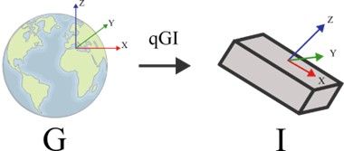
Orientation is arguably one of the most important types of data in biomechanics. However, no sensor can directly measure an object’s orientation relative to a global frame (Figure 1). Therefore, exploring novel algorithms that can compute accurate orientation from a set of input data is a thriving research field with countless applications, including biomechanics, avionics and maritime industries. The sensor fusion algorithms most commonly found in IMU are the Extended or Unscented Kalman Filters (EKF or UKF) and the Complementary Filters (CF). Alternatively, simpler approaches      to compute orientation are the accelerometer+magnetometer method      and gyroscope integration. They     are rarely used in industry due to poor stability, but they compose the basis of modern sensor fusion. In the following paragraph, we provide an overview of each method.

Acc + Mag Method

If the IMU is in a static condition, the accelerometer will measure only the acceleration due to the gravity, hence: . In other words, we have a measure of a constant known vector, the gravity acceleration, in the IMU’s reference frame. In the global frame, the acceleration of gravity is a known vector: and from its measure in the IMU’s frame, we can estimate the orientation of the IMU frame w.r.t. the global frame. On the other hand, when the IMU is in motion, roll and pitch angles can be estimated relatively easily and accurately through trigonometry. For instance, let the orientation vector (roll, pitch and yaw), roll (φ) and pitch (θ) can be estimated from acceleration as shown in (4) and (5).

	(4)
	(5)

However, the accelerometer alone      cannot estimate the full orientation of the IMU frame due to the lack of a horizontal plane reference. In other words, the rotation around the gravity vector (the global z-    axis) is unknown. To compensate for that, the magnetometer establishes a horizontal reference by computing the axis pointing to the magnetic north, given that magnetic disturbances are negligible. By combining the axes from gravity and magnetometer, it is possible to define a direction cosine matrix that can identify the orientation of the IMU with respect to the global frame.

Gyro integration method

As the gyroscope provides an estimate of the IMU’s angular velocity, integrating it over time yields the orientation of the device. However, without prior knowledge of the sensor orientation, the integration can only provide the IMU’s relative orientation in time (e.g. the IMU’s orientation with respect to its previous orientation). Another term to indicate this type of orientation is ‘unreferenced heading’. If the initial orientation is known (or if it’s estimated during a static condition using acc+mag), then the integration of the angular velocity can provide the full orientation of the device. An important downside of this method is the time-related drift due to the integration operation, which increases linearly over time. This makes this method unreliable for long estimations.

Kalman Filters

A Kalman Filter (KF) is the most basic example of a predictive filter. KF uses the initial knowledge of the system, a statistical description of noises and errors and initial measurements of the accelerometer and magnetometer to generate a preliminary system output. This is further updated with gyroscope measurements to redefine the orientation output and reduce the errors. By continuously adjusting these parameters in real-time, the KF can produce an accurate orientation estimate. This method can be further improved in a nonlinear fashion by computing and modelling the acc+mag and gyroscope orientation estimates and relative errors separately. For further information on Kalman Filters, see (Aided Navigation: GPS with High Rate Sensors; Milosevic et al., 2012).

Complementary Filters

The Complementary Filters (CF) approach combines multiple independent noisy measurements of the same signal as long as the noisy terms have complementary spectral characteristics. In the case of the IMU, acc+mag and gyroscope represent two independent orientation estimations with different spectral characteristics. The acc+mag estimation is reliable in static or quasi-static conditions. It is affected by high-frequency noise, whereas the gyroscope estimation is accurate in dynamic conditions but unreliable in static conditions due to the time-integration drift. Therefore, by combining low-frequency information from acc+mag and high-frequency information from the gyroscope, the overall orientation estimation can significantly improve. More detailed information on CF can be found in  (Bachmann, 2000; Madgwick et al., 2011; Mahony et al., 2008).

1.5.                         Translation of reference frames

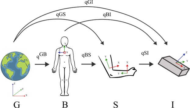
In the previous chapters, we have only referred to the computation of orientation of the IMU with respect to a global reference frame ( if expressed in quaternion format). However, in biomechanics and movement analysis, this type of data yields little meaningful information. What professionals in the medical field look for is the orientation of a body segment with respect to another, or, in other words, a joint angle. To      achieve this, in practical terms, we need to translate the orientation of the sensor (with respect to the global frame) to the orientation of the body segment underneath.  This latter can be expressed to a fixed reference, such as the global frame, or a non-fixed reference, such as the whole body (body frame). Both are meaningful representations of the movement of a body segment in space and are required to compute joint angles. Figure 2 depicts the relationship between the different reference frames and the chain of rotations needed to translate from the global-to-inertial (GI) to the body-to-segment (BS) or global-to-segment (GS) reference frames. The first step to obtain the BS or GS reference frames is to establish a relationship between the body segment and the sensor placed on it. This is referred to as the segment-to-inertial (SI) reference frame (q^SI in Figure 2) and is obtained through the sensor-to-segment calibration that will be discussed in the following paragraphs.

1.6.                            Joint Angles and Anatomical Planes

The last step in obtaining anatomical joint angles is computing the relative orientation between each pair of contiguous proximal-distal body segments. This can be done through quaternion multiplication (if orientation is expressed in quaternion format). For example, in order to compute the elbow joint angles, we need to compute the relative orientation between the upper and lower arm, as displayed in (6) where  represents the Hamilton’s quaternion multiplication and represent the quaternion conjugate. The relative orientation can be expressed in several ways, such as quaternions, rotation matrices or Euler Angles.

(6)

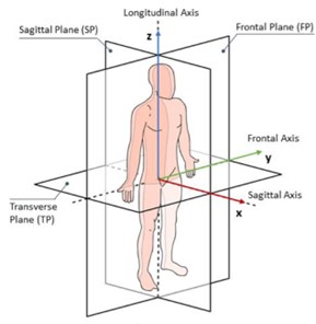
Among these, Euler Angles represent a 3D decomposition of the relative orientation of a pair of segments and are the most commonly found in biomechanics and movement science. They are the easiest way to interpret and understand joint angles, which is of paramount importance in clinical practice, as each angle refers to an anatomical plane of reference and a joint rotation axis. An overview of the anatomical body planes is presented in Figure 3. As in the previous example, the elbow joint can perform flexion/extension, which occurs around the flexion axis and on the sagittal plane, as well as pronation/supination, which occurs around the longitudinal axis and on the transverse plane.

In the last paragraph of this guide, we present a practical guide to computing anatomical joint angles from raw IMU orientation data, as we go through all the steps mentioned above.

2.  Validation and Use in Healthcare

The accuracy of anatomical joint angle computed using pairs of IMU depends on several factors that contribute to the overall error. These can be broadly classified as errors dependent on the accuracy of the orientation of the IMU with respect to a global reference frame (namely Earth) and errors dependent on the quality of the IMU sensor-to-segment alignment. These two sources of error can be quantified,  as described by (Zhu et al., 2023) in their work on shoulder joint angle estimation. On top of this, when IMUs are applied to the human body, other important factors play a role in determining the overall joint angle accuracy. Sensor bias and drift (LaViola, 2003), soft tissue artifacts (Cappello et al., 2005; Cutti et al., 2005; Prabakaran and Rufus, 2022), within-subject repeatability (Charalambous, 2014; Donaldson et al., 2021), to name a few, contribute to skewing the final joint angle readings. For these reasons, validation of the IMU against reference systems becomes of paramount importance for applications in healthcare.  

Given the current state of IMU technology, sensor orientation error is generally low, and most IMU currently on the market can achieve accuracy within 1° on pitch and roll and 3° for the yaw (Jorgensen et al., 2014; McGinnis et al., 2014; Paulich et al., 2018). As described in previous chapters, the differences in accuracy between pitch/roll and yaw are due to the different ways      these angles are calculated. Pitch and roll mostly rely on the accelerometer, which is often reliable, whereas yaw is computed from gyroscope and magnetometer, which are associated with larger errors. On the other hand, sensor-to-segment alignment is the error component that majorly affects anatomical joint angle estimation. This alignment is achieved through a process called sensor-to-segment calibration (or, for brevity, ‘calibration’ in the biomechanics literature), and there are several ways to achieve it. Vitali and Perkins (2020) described in detail all the methods identified in literature, with their relative accuracy. In short, four methods are described: static calibration, where the user holds one or more known postures (generally N-pose or T-pose) for a few seconds (Bonfiglio et al., 2024; Brochard et al., 2011; Zabat et al., 2019); functional calibration, where the user performs one single-plane movement for each degree of freedom of the joint being calibrated (Cottam et al., 2021; de Vries et al., 2010; Favre et al., 2009; Ricci et al., 2014); Assumed alignment or manual alignment (Bonfiglio et al., 2024; Bouvier et al., 2015; Picerno et al., 2019), where the sensors are placed in such a way that a perfect match is assumed between the IMU and the segment reference frames; Augmented methods where machine learning techniques are used to train a model to perform the calibration (Baudet et al., 2014; Chaaban et al., 2021; Fry et al., 2021; McGrath et al., 2018).

IMU that report acceptable accuracy can be used in healthcare applications for a wide range of purposes, including monitoring of biomechanical parameters (Bo et al., 2022; Klaassen et al., 2015; Lyons et al., 2005), assisted rehabilitation (Adans-Dester et al., 2020; Ang, 2018; Belda-Lois et al., 2011), gamification and virtual reality (Ahn et al., 2019; Alankus et al., 2010; Alankus and Kelleher, 2012; Alves et al., 2020) or customized feedback (Bowman et al., 2021). In this toolbox, we discuss a publicly available dataset of IMU data (paired with its optical motion capture data as reference), to facilitate the development of novel algorithms that can boost the use of wearable sensors in healthcare.

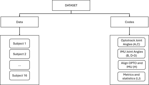
3.  Dataset Description

The full dataset is publicly available at: https://doi.org/10.5281/zenodo.10935873. The dataset contains optical motion capture data and IMU data acquired on 16 subjects throughout a protocol that involves: static pose calibration, functional calibration and a series of single-plane/single-joint and multi-plane/multi-joint upper body exercises (Figure 4). The dataset also contains MATLAB codes and functions to process the raw data for each subject and compute reference metrics to quantify the accuracy of each IMU calibration and statistical analysis (Figure 4). A list with a detailed description of each task and MATLAB script is provided in the readme file within the folder. A version of MATLAB of 2019a or later is recommended to run the scripts.

1.  Toolbox Description

While the Zenodo dataset contains extensive information, explanations and codes to perform a thorough analysis of the data for statistical purposes, as many research dataset, its use might require notable time before one can fully grasp all concepts to compute joint angles from raw IMU data. Furthermore, users far from the research field might get lost in the theory and abandon the exploration of the dataset in favour of quicker or simpler-to-use libraries, leaving little time for learning the concepts. Therefore, we aim to bridge this gap by providing simpler, yet thorough, practical examples to guide a general user with little to no knowledge in biomechanics through the process of computing joint angles from the raw IMU data within the database. Furthermore, we propose a complete Python-based analysis package to lower the entrance barrier to those users who are not familiar with MATLAB or don’t have a license readily available at their institution.

For the sake of brevity, each script analyses data for one subject; however, the same analysis can be repeated for all subjects if required. Since the Zotero database contains MATLAB files, a similar procedure is done in Python to achieve the same results. The system requirements are listed below:

• Python 3.7 or above
• Visual Studio Code Jupiter Notebook extension
• Python libraries required are provided in the ‘requirements.txt’ file

Begin the tutorial by downloading the shared GitHub repository at: https://github.com/alexbonf/Biomechanics-joint-angle-analysis.git

There are several ways to do so:

• Option 1: From the GitHub website go to ‘Code’ 🡪 download ZIP and then place it in a convenient location.
• Option 2: Create a dedicated folder on your drive and from the command line paste (git needs to be installed):

git clone https://github.com/alexbonf/Biomechanics-joint-angle-analysis

Once the folder is stored in your drive, you can run the command below from your command prompt to install all necessary Python libraries.

pip install -r requirements.txt

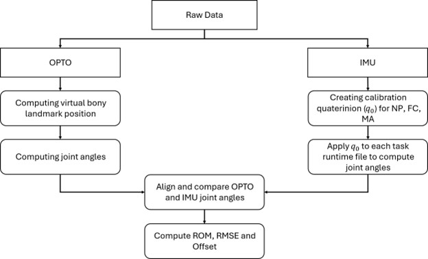
The GitHub folder contains sample data from the full database from subject 1 as well as example Python codes. The general workflow of the scripts presented in this toolbox is graphically represented in Figure 5. The workflow begins with OPTO and IMU data pre-processing, which is different for the two systems. Subsequently, joint angles are computed for both systems, and the timeseries are aligned for comparison. Finally, metrics such as ROM, RMSE and offset are computed for statistical analysis.

4.1.                            Data Exploration

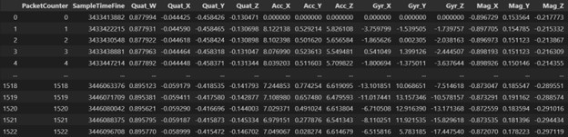
We begin the tutorial by sorting the IMU data and uploading each file in memory, which is done in the first script (1.DataExploration.ipynb). Each csv file contains sampleTimeFine, quaternion, acceleration, gyroscope and magnetometer data (Figure 3). To compute joint angles, we will use quaternions.

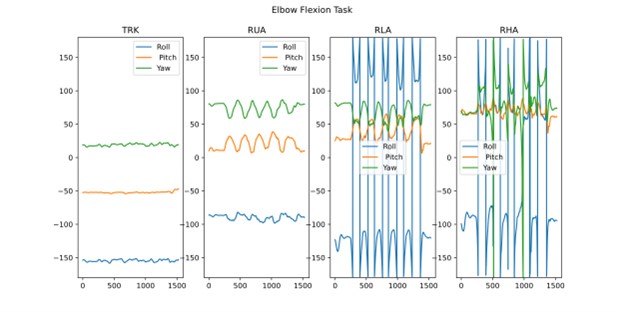
Data is uploaded, stored and saved in a dictionary that will be used in the following scripts to compute      joint angles. Finally, we plot the raw orientation data of each sensor for a given task. The script allows you to play around and choose which task to plot. In the example in Figure 4, the task plotted is an elbow flexion movement. Raw data is generally hard to interpret, and, in this case, Euler angle wrapping occurs making the angle ‘jump’ from -180° to 180°. In order to correctly interpret orientation data, the sensor-to-segment calibration becomes especially important.

4.2.                            IMU Calibration

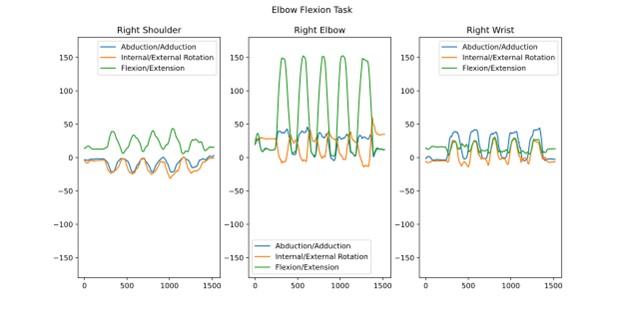
The 2.IMU_calibration.ipynb script computes calibrated joint angles from the static N-pose file.  The first step is computing the qGB (global to body quaternion) from the N-pose calibration file, which is required to compute the qSI (sensor to inertial quaternion). This is addressed in the function ‘compute_qSI’ that uses the trunk sensor rotation matrix during calibration to build a body reference frame with XYZ axes that point forward, up and right respectively. Details on the mathematical operations to compute the qGB and qSI are described in (Bonfiglio et al., 2024). Subsequently, qSI is needed to compute the calibrated segment data qGS (global to segment quaternion), which is addressed in the function ‘compute_calibrated_quaterinons’. Finally, we compute joint angles from the calibrated segment data qGS by performing the quaternion multiplication between each pair of proximal-distal body segments, as described in (6). Joint angles computed in this fashion are easily interpretable and are independent of how the rest of the body is oriented in space. For comparison with Figure 7, Figure 8 displays the same elbow flexion task with shoulder, elbow and wrist joint angle plots. By analysing the elbow flexion angle, the joint movement is easier to visualise and interpret. Note that the overall output of the conversion from quaternion to Euler angles is dependent on the sequence of rotation used. Details on the theory behind Euler sequences can be found in (Karduna et al., 2000; Perumal, 2014; Pio, 1966).

4.3.                            Computing Optical Joint Angles

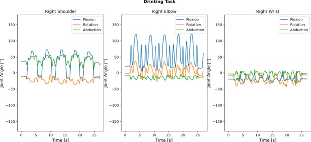
We compute optical motion capture joint angles according to the      International Society of Biomechanics conventions for the upper extremities described in (Wu et al., 2005). We use (virtual) anatomical bony landmark positions to define local reference frames for the trunk, upper arm, lower arm and hand. This process is similar to the IMU joint angle computation; however, in this case, we use the 3D position of the bony landmarks to define 3D vectors that are used to build the rotation matrix of each bony segment reference frame. Since the main focus of the toolbox is on IMU computation, the optical joint angle computation is left relatively simple; however, more extensive algorithms exist in this area. By providing the raw optical c3d data, we let the users explore different computation methods if required. Figure 9 depicts an example of optical motion capture data for all upper limb joints and 3D anatomical axes.

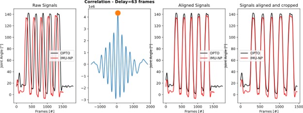
4.4                       Alignment of OPTO and IMU data

To compare OPTO and IMU data, we must ensure a proper time alignment between the two timeseries. We address this issue in the script ‘4.Align_OPTO_IMU_Angles.ipynb’, where we use the point of maximum cross-correlation to identify the time lag between the two systems and perform a time-shift. Figure 10 displays an example of this procedure for the ‘Elbow flexion’ task to align OPTO and IMU data.

4.5.                            Compute Metrics and Statistics

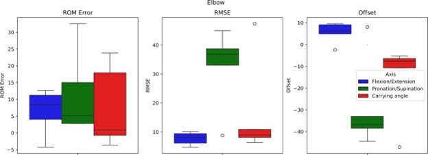
The final part of the analysis is to compute meaningful metrics to compare OPTO and IMU data. We chose the range of motion (ROM) error, Root Mean Squared Error (RMSE) and Offset, as these are most commonly found in biomechanics research and clinical healthcare applications. In the ‘5.OPTO_IMU_Statistics.ipynb’ script, we compute these metrics from the OPTO and IMU data for each joint, task and joint axis on data from one subject and place it in a pandas dataframe. Finally, we plot these metrics as boxplots to provide a graphical overview, as shown in Figure 11. Since this toolbox is intended as a practical exercise, we only include data from one subject. However, if data from more subjects were added, it is possible to run a full statistical analysis to evaluate differences between OPTO and IMU across joints, tasks and axes. For further reading on this topic, see (Bonfiglio et al., 2024)

Conclusions

In this toolbox, we described the working principles of IMU, highlighting methods to estimate orientation and translate it into interpretable joint angles that can be used for biomechanical analysis. Secondly, we discussed general applications of IMU technology in healthcare, and the importance of a thorough validation process against optical reference systems for widespread use in this sector. Thirdly, we introduced a complete dataset publicly available on Zenodo, that features IMU and optical motion capture data collected on 16 subjects across a wide range of upper body tasks. The dataset contains MATLAB codes for data analysis, which was used for the publication of several papers in the field. However, datasets are generally limited to the research world, making it complex and time-     consuming to implement its findings in practical industry applications. Therefore, we aim to bridge this gap by providing a practical guide on the use of IMU to calculate calibrated joint angles from raw orientation data in the last chapter of this toolbox. The data provided in this toolbox is a subset of the Zenodo dataset previously introduced and entirely processed in Python to      lower the entry-     level for the analysis (compared to MATLAB) and provide an open-source environment where users could contribute to improving this analysis. Our ultimate goal is to spread knowledge and awareness on how to use wearable technologies for clinical applications to those with little knowledge of biomechanics and research methods.

References

Adans-Dester, C., Hankov, N., O’Brien, A., Vergara-Diaz, G., Black-Schaffer, R., Zafonte, R., Dy, J., Lee, S.I., Bonato, P., 2020. Enabling precision rehabilitation interventions using wearable sensors and machine learning to track motor recovery. npj Digit. Med. 3, 121. https://doi.org/10.1038/s41746-020-00328-w

Ahn, S., Hwang, S., Ahn, S., Hwang, S., 2019. Virtual rehabilitation of upper extremity function and independence for stoke: a meta-analysis. J Exerc Rehabil 15, 358–369. https://doi.org/10.12965/jer.1938174.087

Aided Navigation: GPS with High Rate Sensors [WWW Document], n.d. URL https://dl.acm.org/doi/10.5555/1594745 (accessed 7.16.24).

Alankus, G., Kelleher, C., 2012. Reducing compensatory motions in video games for stroke rehabilitation, in: Proceedings of the SIGCHI Conference on Human Factors in Computing Systems. Presented at the CHI ’12: CHI Conference on Human Factors in Computing Systems, ACM, Austin Texas USA, pp. 2049–2058. https://doi.org/10.1145/2207676.2208354

Alankus, G., Lazar, A., May, M., Kelleher, C., 2010. Towards customizable games for stroke rehabilitation, in: Proceedings of the SIGCHI Conference on Human Factors in Computing Systems. Presented at the CHI ’10: CHI Conference on Human Factors in Computing Systems, ACM, Atlanta Georgia USA, pp. 2113–2122. https://doi.org/10.1145/1753326.1753649

Alves, T., Carvalho, H., Simões Lopes, D., 2020. Winning compensations: Adaptable gaming approach for upper limb rehabilitation sessions based on compensatory movements. Journal of Biomedical Informatics 108, 103501. https://doi.org/10.1016/j.jbi.2020.103501

Ang, W.S., 2018. A biomechanical model of human upper limb for objective stroke rehabilitation assessment. Nanyang Technological University. https://doi.org/10.32657/10356/73470

Arlotti, J.S., Carroll, W.O., Afifi, Y., Talegaonkar, P., Albuquerque, L., Burch V, R.F., Ball, J.E., Chander, H., Petway, A., 2022. Benefits of IMU-based Wearables in Sports Medicine: Narrative Review. IJKSS 10, 36–43. https://doi.org/10.7575/aiac.ijkss.v.10n.1p.36

Bachmann, E.R., 2000. INERTIAL AND MAGNETIC TRACKING OF LIMB SEGMENT ORIENTATION FOR INSERTING HUMANS INTO SYNTHETIC ENVIRONMENTS.

Baudet, A., Morisset, C., d’Athis, P., Maillefert, J.-F., Casillas, J.-M., Ornetti, P., Laroche, D., 2014. Cross-Talk Correction Method for Knee Kinematics in Gait Analysis Using Principal Component Analysis (PCA): A New Proposal. PLoS ONE 9, e102098. https://doi.org/10.1371/journal.pone.0102098

Belda-Lois, J.-M., Mena-del Horno, S., Bermejo-Bosch, I., Moreno, J.C., Pons, J.L., Farina, D., Iosa, M., Molinari, M., Tamburella, F., Ramos, A., Caria, A., Solis-Escalante, T., Brunner, C., Rea, M., 2011. Rehabilitation of gait after stroke: a review towards a top-down approach. J NeuroEngineering Rehabil 8, 66. https://doi.org/10.1186/1743-0003-8-66

Bo, F., Yerebakan, M., Dai, Y., Wang, W., Li, J., Hu, B., Gao, S., 2022. IMU-Based Monitoring for Assistive Diagnosis and Management of IoHT: A Review. Healthcare 10, 1210. https://doi.org/10.3390/healthcare10071210

Bonfiglio, A., Tacconi, D., Bongers, R.M., Farella, E., 2024. Effects of IMU sensor-to-segment calibration on clinical 3D elbow joint angles estimation. Front. Bioeng. Biotechnol. 12, 1385750. https://doi.org/10.3389/fbioe.2024.1385750

Bouvier, B., Duprey, S., Claudon, L., Dumas, R., Savescu, A., 2015. Upper Limb Kinematics Using Inertial and Magnetic Sensors: Comparison of Sensor-to-Segment Calibrations. Sensors 15, 18813–18833. https://doi.org/10.3390/s150818813

Bowman, T., Gervasoni, E., Arienti, C., Lazzarini, S., Negrini, S., Crea, S., Cattaneo, D., Carrozza, M., 2021. Wearable Devices for Biofeedback Rehabilitation: A Systematic Review and Meta-Analysis to Design Application Rules and Estimate the Effectiveness on Balance and Gait Outcomes in Neurological Diseases. Sensors 21, 3444. https://doi.org/10.3390/s21103444

Brochard, S., Lempereur, M., Rémy-Néris, O., 2011. Double calibration: An accurate, reliable and easy-to-use method for 3D scapular motion analysis. Journal of Biomechanics 44, 751–754. https://doi.org/10.1016/j.jbiomech.2010.11.017

Cappello, A., Stagni, R., Fantozzi, S., Leardini, A., 2005. Soft Tissue Artifact Compensation in Knee Kinematics by Double Anatomical Landmark Calibration: Performance of a Novel Method During Selected Motor Tasks. IEEE Trans. Biomed. Eng. 52, 992–998. https://doi.org/10.1109/TBME.2005.846728

Chaaban, C.R., Berry, N.T., Armitano-Lago, C., Kiefer, A.W., Mazzoleni, M.J., Padua, D.A., 2021. Combining Inertial Sensors and Machine Learning to Predict vGRF and Knee Biomechanics during a Double Limb Jump Landing Task. Sensors 21, 4383. https://doi.org/10.3390/s21134383

Charalambous, C.P., 2014. Repeatability of Kinematic, Kinetic, and Electromyographic Data in Normal Adult Gait, in: Banaszkiewicz, P.A., Kader, D.F. (Eds.), Classic Papers in Orthopaedics. Springer London, London, pp. 399–401. https://doi.org/10.1007/978-1-4471-5451-8_101

Cottam, D.S., Campbell, A.C., Davey, P.C., Kent, P., Elliott, B.C., Alderson, J.A., 2021. Functional calibration does not improve the concurrent validity of magneto-inertial wearable sensor-based thorax and lumbar angle measurements when compared with retro-reflective motion capture. Med Biol Eng Comput 59, 2253–2262. https://doi.org/10.1007/s11517-021-02440-9

Cutti, A.G., Cappello, A., Davalli, A., 2005. A new technique for compensating the soft tissue artefact at the upper-arm: in vitro validation. J. Mech. Med. Biol. 05, 333–347. https://doi.org/10.1142/S0219519405001485

de Vries, W.H.K., Veeger, H.E.J., Cutti, A.G., Baten, C., van der Helm, F.C.T., 2010. Functionally interpretable local coordinate systems for the upper extremity using inertial & magnetic measurement systems. Journal of Biomechanics 43, 1983–1988. https://doi.org/10.1016/j.jbiomech.2010.03.007

Donaldson, B., Bezodis, N., Bayne, H., 2021. WITHIN-SUBJECT REPEATABILITY AND BETWEEN-SUBJECT VARIABILITY IN POSTURE DURING CALIBRATION OF AN INERTIAL MEASUREMENT UNIT SYSTEM.

Favre, J., Aissaoui, R., Jolles, B.M., de Guise, J.A., Aminian, K., 2009. Functional calibration procedure for 3D knee joint angle description using inertial sensors. Journal of Biomechanics 42, 2330–2335. https://doi.org/10.1016/j.jbiomech.2009.06.025

Fry, K.E., Chen, Y.-P., Howard, A., 2021. Method for the Determination of Relative Joint Axes for Wearable Inertial Sensor Applications, in: 2021 IEEE/RSJ International Conference on Intelligent Robots and Systems (IROS). Presented at the 2021 IEEE/RSJ International Conference on Intelligent Robots and Systems (IROS), IEEE, Prague, Czech Republic, pp. 9512–9517. https://doi.org/10.1109/IROS51168.2021.9636686

Inertial Measurement Units (IMU) – iNEMO inertial sensors and modules – STMicroelectronics [WWW Document], n.d. URL https://www.st.com/en/mems-and-sensors/inemo-inertial-modules.html (accessed 7.16.24).

Jorgensen, M.J., Paccagnan, D., Poulsen, N.K., Larsen, M.B., 2014. IMU calibration and validation in a factory, remote on land and at sea, in: 2014 IEEE/ION Position, Location and Navigation Symposium – PLANS 2014. Presented at the 2014 IEEE/ION Position, Location and Navigation Symposium – PLANS 2014, IEEE, Monterey, CA, pp. 1384–1391. https://doi.org/10.1109/PLANS.2014.6851514

Karduna, A.R., McClure, P.W., Michener, L.A., 2000. Scapular kinematics: e!ects of altering the Euler angle sequence of rotations. Journal of Biomechanics.

Klaassen, B., Van Beijnum, B.-J., Weusthof, M., Hofs, D., Van Meulen, F., Droog, E., Luinge, H., Slot, L., Tognetti, A., Lorussi, F., Paradiso, R., Held, J., Luft, A., Reenalda, J., Nikamp, C., Buurke, J., Hermens, H., Veltink, P., 2015. A Full Body Sensing System for Monitoring Stroke Patients in a Home Environment, in: Plantier, G., Schultz, T., Fred, A., Gamboa, H. (Eds.), Biomedical Engineering Systems and Technologies, Communications in Computer and Information Science. Springer International Publishing, Cham, pp. 378–393. https://doi.org/10.1007/978-3-319-26129-4_25

LaViola, J.J., 2003. A comparison of unscented and extended Kalman filtering for estimating quaternion motion, in: Proceedings of the 2003 American Control Conference, 2003. Presented at the 2003 American Control Conference, IEEE, Denver, CO, USA, pp. 2435–2440. https://doi.org/10.1109/ACC.2003.1243440

Lyons, G.M., Culhane, K.M., Hilton, D., Grace, P.A., Lyons, D., 2005. A description of an accelerometer-based mobility monitoring technique. Medical Engineering & Physics 27, 497–504. https://doi.org/10.1016/j.medengphy.2004.11.006

Madgwick, S.O.H., Harrison, A.J.L., Vaidyanathan, R., 2011. Estimation of IMU and MARG orientation using a gradient descent algorithm, in: 2011 IEEE International Conference on Rehabilitation Robotics. Presented at the 2011 IEEE 12th International Conference on Rehabilitation Robotics: Reaching Users & the Community (ICORR 2011), IEEE, Zurich, pp. 1–7. https://doi.org/10.1109/ICORR.2011.5975346

Mahony, R., Hamel, T., Pflimlin, J.-M., 2008. Nonlinear Complementary Filters on the Special Orthogonal Group. IEEE Trans. Automat. Contr. 53, 1203–1218. https://doi.org/10.1109/TAC.2008.923738

McGinnis, R.S., Cain, S.M., Davidson, S.P., Vitali, R.V., McLean, S.G., Perkins, N.C., 2014. Validation of Complementary Filter Based IMU Data Fusion for Tracking Torso Angle and Rifle Orientation, in: Volume 3: Biomedical and Biotechnology Engineering. Presented at the ASME 2014 International Mechanical Engineering Congress and Exposition, American Society of Mechanical Engineers, Montreal, Quebec, Canada, p. V003T03A052. https://doi.org/10.1115/IMECE2014-36909

McGrath, T., Fineman, R., Stirling, L., 2018. An Auto-Calibrating Knee Flexion-Extension Axis Estimator Using Principal Component Analysis with Inertial Sensors 17.

Milosevic, B., Naldi, R., Farella, E., Benini, L., Marconi, L., 2012. Design and validation of an attitude and heading reference system for an aerial robot prototype, in: 2012 American Control Conference (ACC). Presented at the 2012 American Control Conference – ACC 2012, IEEE, Montreal, QC, pp. 1720–1725. https://doi.org/10.1109/ACC.2012.6314975

MPU-9250 | TDK InvenSense [WWW Document], n.d. URL https://invensense.tdk.com/products/motion-tracking/9-axis/mpu-9250/ (accessed 7.16.24).

Paulich, M., Schepers, M., Rudigkeit, N., Bellusci, G., 2018. Xsens MTw Awinda: Miniature Wireless Inertial-Magnetic Motion Tracker for Highly Accurate 3D Kinematic Applications.

Perumal, L., 2014. Euler angles: conversion of arbitrary rotation sequences to specific rotation sequence. Computer Animation & Virtual 25, 521–529. https://doi.org/10.1002/cav.1529

Picerno, P., Caliandro, P., Iacovelli, C., Simbolotti, C., Crabolu, M., Pani, D., Vannozzi, G., Reale, G., Rossini, P.M., Padua, L., Cereatti, A., 2019. Upper limb joint kinematics using wearable magnetic and inertial measurement units: an anatomical calibration procedure based on bony landmark identification. Sci Rep 9, 14449. https://doi.org/10.1038/s41598-019-50759-z

Pio, R., 1966. Euler angle transformations. IEEE Trans. Automat. Contr. 11, 707–715. https://doi.org/10.1109/TAC.1966.1098430

Prabakaran, A., Rufus, E., 2022. Review on the wearable health-care monitoring system with robust motion artifacts reduction techniques. SR 42, 19–38. https://doi.org/10.1108/SR-05-2021-0150

Ricci, L., Formica, D., Sparaci, L., Lasorsa, F., Taffoni, F., Tamilia, E., Guglielmelli, E., 2014. A New Calibration Methodology for Thorax and Upper Limbs Motion Capture in Children Using Magneto and Inertial Sensors. Sensors 14, 1057–1072. https://doi.org/10.3390/s140101057

Vitali, R.V., Perkins, N.C., 2020. Determining anatomical frames via inertial motion capture: A survey of methods. Journal of Biomechanics 106, 109832. https://doi.org/10.1016/j.jbiomech.2020.109832

Williamson, J., Qi Liu, Fenglong Lu, Mohrman, W., Kun Li, Dick, R., Li Shang, 2015. Data sensing and analysis: Challenges for wearables, in: The 20th Asia and South Pacific Design Automation Conference. Presented at the 2015 20th Asia and South Pacific Design Automation Conference (ASP-DAC), IEEE, Chiba, Japan, pp. 136–141. https://doi.org/10.1109/ASPDAC.2015.7058994

Wu, G., van der Helm, F.C.T., (DirkJan) Veeger, H.E.J., Makhsous, M., Van Roy, P., Anglin, C., Nagels, J., Karduna, A.R., McQuade, K., Wang, X., Werner, F.W., Buchholz, B., 2005. ISB recommendation on definitions of joint coordinate systems of various joints for the reporting of human joint motion—Part II: shoulder, elbow, wrist and hand. Journal of Biomechanics 38, 981–992. https://doi.org/10.1016/j.jbiomech.2004.05.042

Zabat, M., Ababou, A., Ababou, N., Dumas, R., 2019. IMU-based sensor-to-segment multiple calibration for upper limb joint angle measurement—a proof of concept. Med Biol Eng Comput 12.

Zhu, K., Li, J., Li, D., Fan, B., Shull, P.B., 2023. IMU Shoulder Angle Estimation: Effects of Sensor-to-Segment Misalignment and Sensor Orientation Error. IEEE Trans. Neural Syst. Rehabil. Eng. 31, 4481–4491. https://doi.org/10.1109/TNSRE.2023.3331238